Prediction (out of sample)
[1]:
%matplotlib inline
[2]:
import numpy as np
import statsmodels.api as sm
Artificial data
[3]:
nsample = 50
sig = 0.25
x1 = np.linspace(0, 20, nsample)
X = np.column_stack((x1, np.sin(x1), (x1-5)**2))
X = sm.add_constant(X)
beta = [5., 0.5, 0.5, -0.02]
y_true = np.dot(X, beta)
y = y_true + sig * np.random.normal(size=nsample)
Estimation
[4]:
olsmod = sm.OLS(y, X)
olsres = olsmod.fit()
print(olsres.summary())
                            OLS Regression Results
==============================================================================
Dep. Variable:                      y   R-squared:                       0.989
Model:                            OLS   Adj. R-squared:                  0.988
Method:                 Least Squares   F-statistic:                     1326.
Date:                Tue, 17 Dec 2019   Prob (F-statistic):           1.18e-44
Time:                        23:39:41   Log-Likelihood:                 8.4408
No. Observations:                  50   AIC:                            -8.882
Df Residuals:                      46   BIC:                            -1.234
Df Model:                           3
Covariance Type:            nonrobust
==============================================================================
                 coef    std err          t      P>|t|      [0.025      0.975]
------------------------------------------------------------------------------
const          4.8426      0.073     66.676      0.000       4.696       4.989
x1             0.5258      0.011     46.943      0.000       0.503       0.548
x2             0.5333      0.044     12.111      0.000       0.445       0.622
x3            -0.0219      0.001    -22.256      0.000      -0.024      -0.020
==============================================================================
Omnibus:                        3.262   Durbin-Watson:                   2.218
Prob(Omnibus):                  0.196   Jarque-Bera (JB):                2.222
Skew:                          -0.402   Prob(JB):                        0.329
Kurtosis:                       3.648   Cond. No.                         221.
==============================================================================

Warnings:
[1] Standard Errors assume that the covariance matrix of the errors is correctly specified.
In-sample prediction
[5]:
ypred = olsres.predict(X)
print(ypred)
[ 4.29539098  4.80736761  5.27727471  5.67604936  5.98511733  6.19944471
  6.32836499  6.3940456   6.42784586  6.46516473  6.53962487  6.6775485
  6.8936328   7.18853511  7.54876503  7.94890079  8.35576599  8.7338804
  9.05128925  9.2848133   9.42385717  9.47215005  9.44713309  9.37709381
  9.29651856  9.24042651  9.23861612  9.31076928  9.46321769  9.68790257
  9.96369866 10.25988507 10.54119263 10.77359851 10.92991608 10.9942616
 10.96466386 10.85338805 10.68492063 10.49194626 10.30997784 10.17152178
 10.10073735 10.10946733 10.19529231 10.34192817 10.52190155 10.70106359
 10.84420053 10.92081924]
Create a new sample of explanatory variables Xnew, predict and plot
[6]:
x1n = np.linspace(20.5,25, 10)
Xnew = np.column_stack((x1n, np.sin(x1n), (x1n-5)**2))
Xnew = sm.add_constant(Xnew)
ynewpred =  olsres.predict(Xnew) # predict out of sample
print(ynewpred)
[10.89466562 10.72741816 10.43998979 10.08003848  9.71029886  9.39322261
  9.17568813  9.07752305  9.08664973  9.16204231]
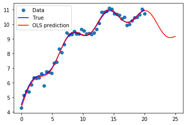
Plot comparison
[7]:
import matplotlib.pyplot as plt

fig, ax = plt.subplots()
ax.plot(x1, y, 'o', label="Data")
ax.plot(x1, y_true, 'b-', label="True")
ax.plot(np.hstack((x1, x1n)), np.hstack((ypred, ynewpred)), 'r', label="OLS prediction")
ax.legend(loc="best");
Predicting with Formulas
Using formulas can make both estimation and prediction a lot easier
[8]:
from statsmodels.formula.api import ols

data = {"x1" : x1, "y" : y}

res = ols("y ~ x1 + np.sin(x1) + I((x1-5)**2)", data=data).fit()
We use the I to indicate use of the Identity transform. Ie., we do not want any expansion magic from using **2
[9]:
res.params
[9]:
Intercept           4.842590
x1                  0.525808
np.sin(x1)          0.533273
I((x1 - 5) ** 2)   -0.021888
dtype: float64
Now we only have to pass the single variable and we get the transformed right-hand side variables automatically
[10]:
res.predict(exog=dict(x1=x1n))
[10]:
0    10.894666
1    10.727418
2    10.439990
3    10.080038
4     9.710299
5     9.393223
6     9.175688
7     9.077523
8     9.086650
9     9.162042
dtype: float64