statsmodels.tsa.filters.cf_filter.cffilter¶

statsmodels.tsa.filters.cf_filter.cffilter(x, low=6, high=32, drift=True)[source]¶

Christiano Fitzgerald asymmetric, random walk filter.

Parameters

xarray_like: The 1 or 2d array to filter. If 2d, variables are assumed to be in columns.
lowfloat: Minimum period of oscillations. Features below low periodicity are filtered out. Default is 6 for quarterly data, giving a 1.5 year periodicity.
highfloat: Maximum period of oscillations. Features above high periodicity are filtered out. Default is 32 for quarterly data, giving an 8 year periodicity.
driftbool: Whether or not to remove a trend from the data. The trend is estimated as np.arange(nobs)*(x[-1] - x[0])/(len(x)-1).

Returns

cyclearray_like: The features of x between the periodicities low and high.
trendarray_like: The trend in the data with the cycles removed.

See also

statsmodels.tsa.filters.bk_filter.bkfilter: Baxter-King filter.
statsmodels.tsa.filters.bk_filter.hpfilter: Hodrick-Prescott filter.
statsmodels.tsa.seasonal.seasonal_decompose: Decompose a time series using moving averages.
statsmodels.tsa.seasonal.STL: Season-Trend decomposition using LOESS.

Examples

>>> dta = sm.datasets.macrodata.load_pandas().data
>>> index = pd.DatetimeIndex(start='1959Q1', end='2009Q4', freq='Q')
>>> dta.set_index(index, inplace=True)

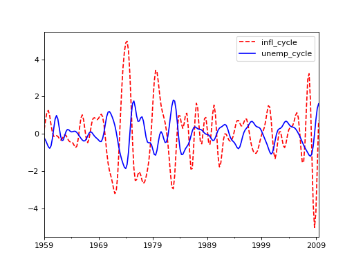
>>> cf_cycles, cf_trend = sm.tsa.filters.cffilter(dta[["infl", "unemp"]])

>>> import matplotlib.pyplot as plt
>>> fig, ax = plt.subplots()
>>> cf_cycles.plot(ax=ax, style=['r--', 'b-'])
>>> plt.show()

(Source code, png, hires.png, pdf)