
Vector Autoregressions tsa.vector_ar
VAR(p) processes
We are interested in modeling a \(T \times K\) multivariate time series \(Y\), where \(T\) denotes the number of observations and \(K\) the number of variables. One way of estimating relationships between the time series and their lagged values is the vector autoregression process:
where \(A_i\) is a \(K \times K\) coefficient matrix.
We follow in large part the methods and notation of Lutkepohl (2005), which we will not develop here.
Model fitting
Note
The classes referenced below are accessible via the
statsmodels.tsa.api module.
To estimate a VAR model, one must first create the model using an ndarray of homogeneous or structured dtype. When using a structured or record array, the class will use the passed variable names. Otherwise they can be passed explicitly:
 # some example data
In [1]: import numpy as np

In [2]: import pandas

In [3]: import statsmodels.api as sm

In [4]: from statsmodels.tsa.api import VAR, DynamicVAR

In [5]: mdata = sm.datasets.macrodata.load_pandas().data

 # prepare the dates index
In [6]: dates = mdata[['year', 'quarter']].astype(int).astype(str)

In [7]: quarterly = dates["year"] + "Q" + dates["quarter"]

In [8]: from statsmodels.tsa.base.datetools import dates_from_str

In [9]: quarterly = dates_from_str(quarterly)

In [10]: mdata = mdata[['realgdp','realcons','realinv']]

In [11]: mdata.index = pandas.DatetimeIndex(quarterly)

In [12]: data = np.log(mdata).diff().dropna()

 # make a VAR model
In [13]: model = VAR(data)
Note
The VAR class assumes that the passed time series are
stationary. Non-stationary or trending data can often be transformed to be
stationary by first-differencing or some other method. For direct analysis of
non-stationary time series, a standard stable VAR(p) model is not
appropriate.
To actually do the estimation, call the fit method with the desired lag order. Or you can have the model select a lag order based on a standard information criterion (see below):
In [14]: results = model.fit(2)

In [15]: results.summary()
Out[15]:
  Summary of Regression Results
==================================
Model:                         VAR
Method:                        OLS
Date:           Mon, 14, May, 2018
Time:                     21:48:15
--------------------------------------------------------------------
No. of Equations:         3.00000    BIC:                   -27.5830
Nobs:                     200.000    HQIC:                  -27.7892
Log likelihood:           1962.57    FPE:                7.42129e-13
AIC:                     -27.9293    Det(Omega_mle):     6.69358e-13
--------------------------------------------------------------------
Results for equation realgdp
==============================================================================
                 coefficient       std. error           t-stat            prob
------------------------------------------------------------------------------
const               0.001527         0.001119            1.365           0.172
L1.realgdp         -0.279435         0.169663           -1.647           0.100
L1.realcons         0.675016         0.131285            5.142           0.000
L1.realinv          0.033219         0.026194            1.268           0.205
L2.realgdp          0.008221         0.173522            0.047           0.962
L2.realcons         0.290458         0.145904            1.991           0.047
L2.realinv         -0.007321         0.025786           -0.284           0.776
==============================================================================

Results for equation realcons
==============================================================================
                 coefficient       std. error           t-stat            prob
------------------------------------------------------------------------------
const               0.005460         0.000969            5.634           0.000
L1.realgdp         -0.100468         0.146924           -0.684           0.494
L1.realcons         0.268640         0.113690            2.363           0.018
L1.realinv          0.025739         0.022683            1.135           0.257
L2.realgdp         -0.123174         0.150267           -0.820           0.412
L2.realcons         0.232499         0.126350            1.840           0.066
L2.realinv          0.023504         0.022330            1.053           0.293
==============================================================================

Results for equation realinv
==============================================================================
                 coefficient       std. error           t-stat            prob
------------------------------------------------------------------------------
const              -0.023903         0.005863           -4.077           0.000
L1.realgdp         -1.970974         0.888892           -2.217           0.027
L1.realcons         4.414162         0.687825            6.418           0.000
L1.realinv          0.225479         0.137234            1.643           0.100
L2.realgdp          0.380786         0.909114            0.419           0.675
L2.realcons         0.800281         0.764416            1.047           0.295
L2.realinv         -0.124079         0.135098           -0.918           0.358
==============================================================================

Correlation matrix of residuals
             realgdp  realcons   realinv
realgdp     1.000000  0.603316  0.750722
realcons    0.603316  1.000000  0.131951
realinv     0.750722  0.131951  1.000000
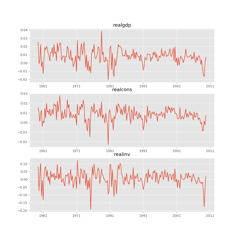
Several ways to visualize the data using matplotlib are available.
Plotting input time series:
In [16]: results.plot()
Out[16]: <Figure size 1000x1000 with 3 Axes>
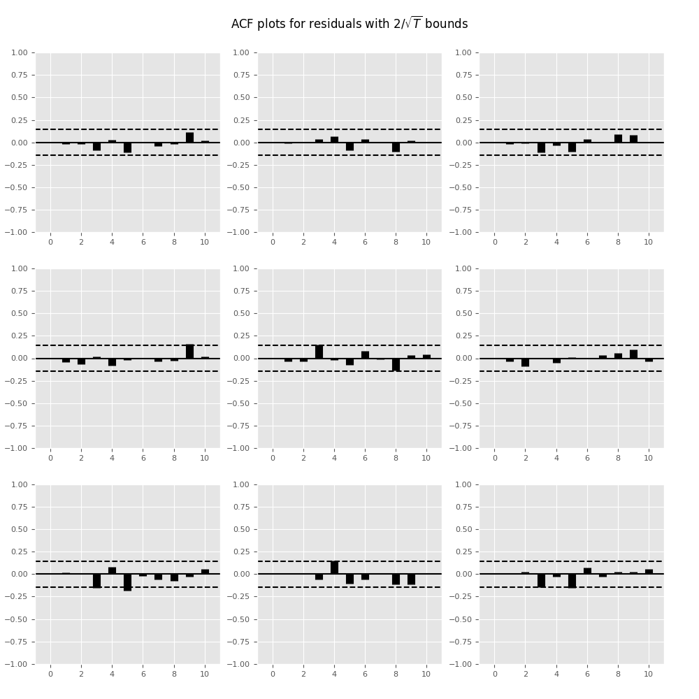
Plotting time series autocorrelation function:
In [17]: results.plot_acorr()
Out[17]: <Figure size 1000x1000 with 9 Axes>
Lag order selection
Choice of lag order can be a difficult problem. Standard analysis employs
likelihood test or information criteria-based order selection. We have
implemented the latter, accessible through the VAR class:
In [18]: model.select_order(15)
Out[18]: <statsmodels.tsa.vector_ar.var_model.LagOrderResults at 0x10c89fef0>
When calling the fit function, one can pass a maximum number of lags and the order criterion to use for order selection:
In [19]: results = model.fit(maxlags=15, ic='aic')
Forecasting
The linear predictor is the optimal h-step ahead forecast in terms of mean-squared error:
We can use the forecast function to produce this forecast. Note that we have to specify the “initial value” for the forecast:
In [20]: lag_order = results.k_ar

In [21]: results.forecast(data.values[-lag_order:], 5)
Out[21]:
array([[ 0.0062,  0.005 ,  0.0092],
       [ 0.0043,  0.0034, -0.0024],
       [ 0.0042,  0.0071, -0.0119],
       [ 0.0056,  0.0064,  0.0015],
       [ 0.0063,  0.0067,  0.0038]])
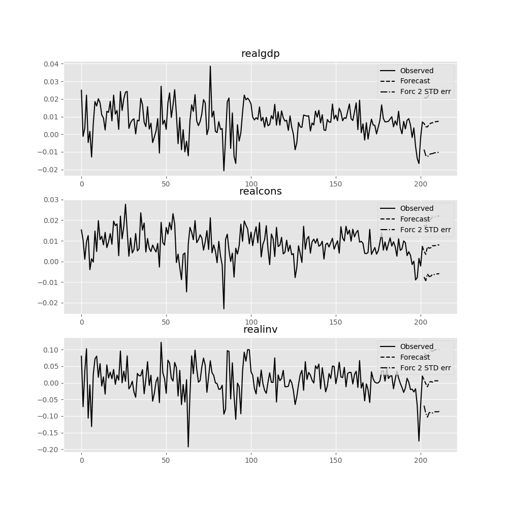
The forecast_interval function will produce the above forecast along with asymptotic standard errors. These can be visualized using the plot_forecast function:
In [22]: results.plot_forecast(10)
Out[22]: <Figure size 1000x1000 with 3 Axes>
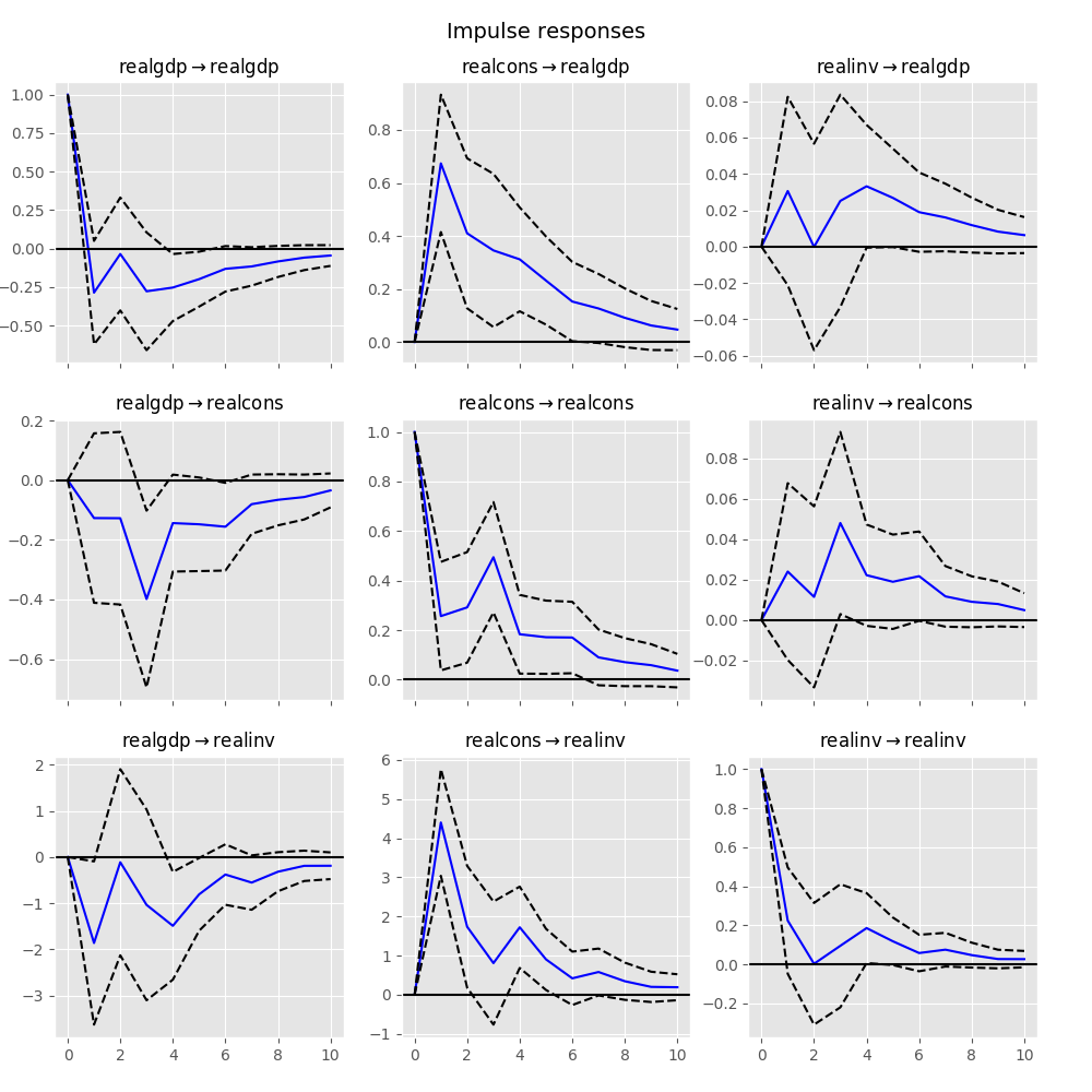
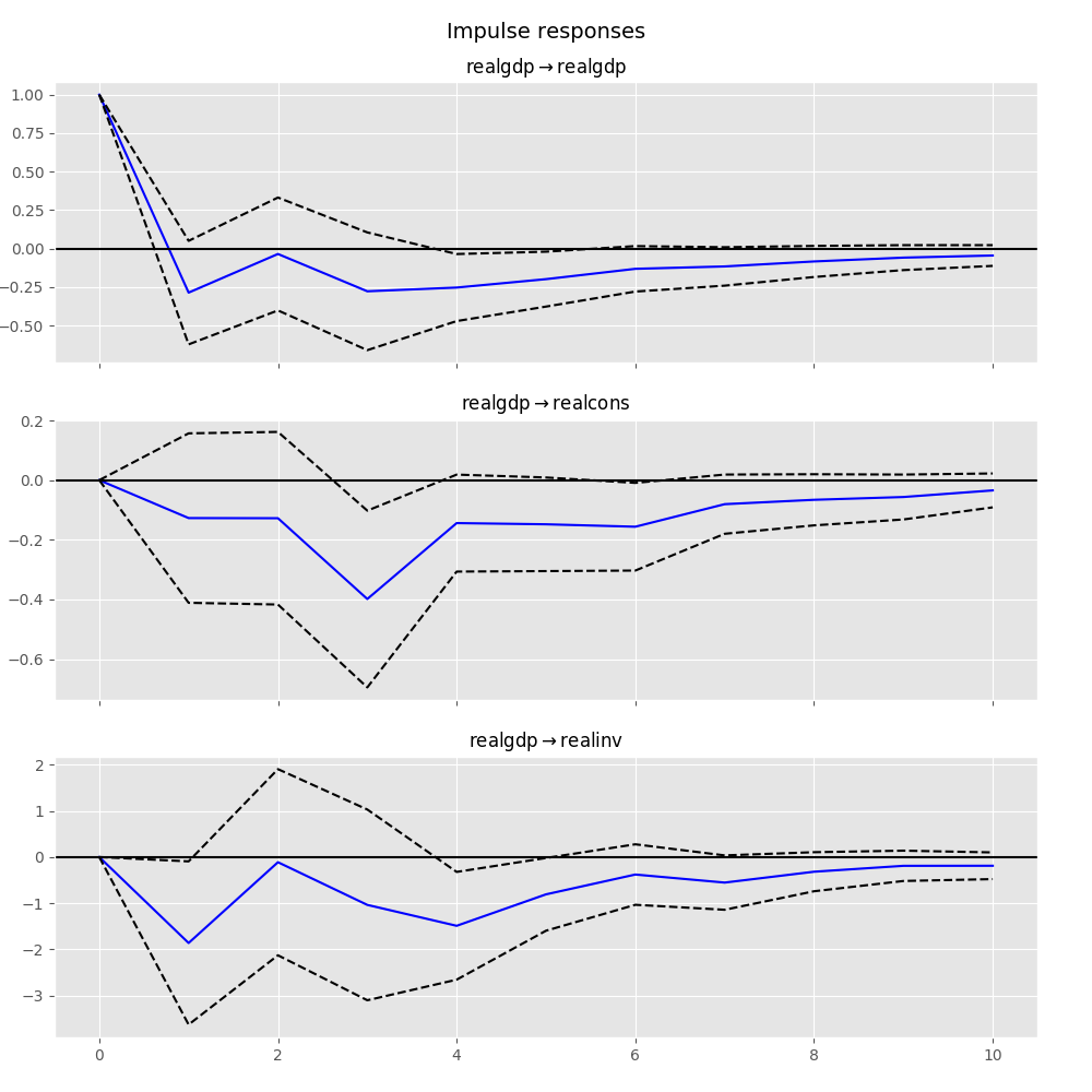
Impulse Response Analysis
Impulse responses are of interest in econometric studies: they are the estimated responses to a unit impulse in one of the variables. They are computed in practice using the MA(\(\infty\)) representation of the VAR(p) process:
We can perform an impulse response analysis by calling the irf function on a VARResults object:
In [23]: irf = results.irf(10)
These can be visualized using the plot function, in either orthogonalized or non-orthogonalized form. Asymptotic standard errors are plotted by default at the 95% significance level, which can be modified by the user.
Note
Orthogonalization is done using the Cholesky decomposition of the estimated error covariance matrix \(\hat \Sigma_u\) and hence interpretations may change depending on variable ordering.
In [24]: irf.plot(orth=False)
Out[24]: <Figure size 1000x1000 with 9 Axes>
Note the plot function is flexible and can plot only variables of interest if so desired:
In [25]: irf.plot(impulse='realgdp')
Out[25]: <Figure size 1000x1000 with 3 Axes>
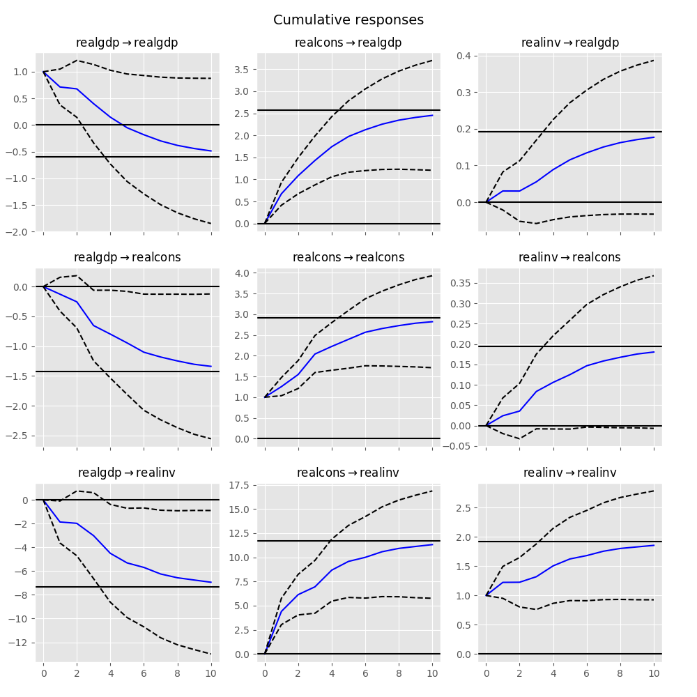
The cumulative effects \(\Psi_n = \sum_{i=0}^n \Phi_i\) can be plotted with the long run effects as follows:
In [26]: irf.plot_cum_effects(orth=False)
Out[26]: <Figure size 1000x1000 with 9 Axes>
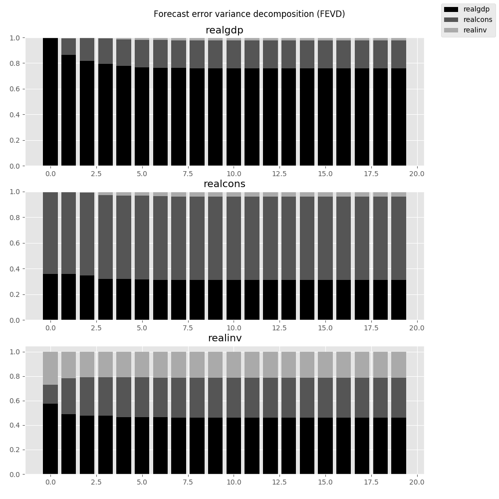
Forecast Error Variance Decomposition (FEVD)
Forecast errors of component j on k in an i-step ahead forecast can be decomposed using the orthogonalized impulse responses \(\Theta_i\):
These are computed via the fevd function up through a total number of steps ahead:
In [27]: fevd = results.fevd(5)

In [28]: fevd.summary()
FEVD for realgdp
      realgdp  realcons   realinv
0    1.000000  0.000000  0.000000
1    0.864889  0.129253  0.005858
2    0.816725  0.177898  0.005378
3    0.793647  0.197590  0.008763
4    0.777279  0.208127  0.014594

FEVD for realcons
      realgdp  realcons   realinv
0    0.359877  0.640123  0.000000
1    0.358767  0.635420  0.005813
2    0.348044  0.645138  0.006817
3    0.319913  0.653609  0.026478
4    0.317407  0.652180  0.030414

FEVD for realinv
      realgdp  realcons   realinv
0    0.577021  0.152783  0.270196
1    0.488158  0.293622  0.218220
2    0.478727  0.314398  0.206874
3    0.477182  0.315564  0.207254
4    0.466741  0.324135  0.209124
They can also be visualized through the returned FEVD object:
In [29]: results.fevd(20).plot()
Out[29]: <Figure size 1000x1000 with 3 Axes>
Statistical tests
A number of different methods are provided to carry out hypothesis tests about the model results and also the validity of the model assumptions (normality, whiteness / “iid-ness” of errors, etc.).
Granger causality
One is often interested in whether a variable or group of variables is “causal”
for another variable, for some definition of “causal”. In the context of VAR
models, one can say that a set of variables are Granger-causal within one of the
VAR equations. We will not detail the mathematics or definition of Granger
causality, but leave it to the reader. The VARResults object has the
test_causality method for performing either a Wald (\(\chi^2\)) test or an
F-test.
In [30]: results.test_causality('realgdp', ['realinv', 'realcons'], kind='f')
Out[30]: <statsmodels.tsa.vector_ar.hypothesis_test_results.CausalityTestResults at 0x10ca15978>
Normality
Whiteness of residuals
Dynamic Vector Autoregressions
Note
To use this functionality, pandas must be installed. See the pandas documentation for more information on the below data structures.
One is often interested in estimating a moving-window regression on time series data for the purposes of making forecasts throughout the data sample. For example, we may wish to produce the series of 2-step-ahead forecasts produced by a VAR(p) model estimated at each point in time.
In [31]: np.random.seed(1)

In [32]: import pandas.util.testing as ptest

In [33]: ptest.N = 500

In [34]: data = ptest.makeTimeDataFrame().cumsum(0)

In [35]: data
Out[35]:
                    A          B          C          D
2000-01-03   1.624345  -1.719394  -0.153236   1.301225
2000-01-04   1.012589  -1.662273  -2.585745   0.988833
2000-01-05   0.484417  -2.461821  -2.077760   0.717604
2000-01-06  -0.588551  -2.753416  -2.401793   2.580517
2000-01-07   0.276856  -3.012398  -3.912869   1.937644
...               ...        ...        ...        ...
2001-11-26  29.552085  14.274036  39.222558 -13.243907
2001-11-27  30.080964  11.996738  38.589968 -12.682989
2001-11-28  27.843878  11.927114  38.380121 -13.604648
2001-11-29  26.736165  12.280984  40.277282 -12.957273
2001-11-30  26.718447  12.094029  38.895890 -11.570447

[500 rows x 4 columns]

In [36]: var = DynamicVAR(data, lag_order=2, window_type='expanding')
The estimated coefficients for the dynamic model are returned as a
pandas.Panel object, which can allow you to easily examine, for
example, all of the model coefficients by equation or by date:
In [37]: import datetime as dt
In [38]: var.coefs
Out[38]:
<class 'pandas.core.panel.Panel'>
Dimensions: 9 (items) x 489 (major_axis) x 4 (minor_axis)
Items axis: L1.A to intercept
Major_axis axis: 2000-01-18 00:00:00 to 2001-11-30 00:00:00
Minor_axis axis: A to D
# all estimated coefficients for equation A
In [39]: var.coefs.minor_xs('A').info()
������������������������������������������������������������������������������������������������������������������������������������������������������������������������������������������������������������������������<class 'pandas.core.frame.DataFrame'>
DatetimeIndex: 489 entries, 2000-01-18 to 2001-11-30
Freq: B
Data columns (total 9 columns):
L1.A 489 non-null float64
L1.B 489 non-null float64
L1.C 489 non-null float64
L1.D 489 non-null float64
L2.A 489 non-null float64
L2.B 489 non-null float64
L2.C 489 non-null float64
L2.D 489 non-null float64
intercept 489 non-null float64
dtypes: float64(9)
memory usage: 58.2 KB
# coefficients on 11/30/2001
In [40]: var.coefs.major_xs(dt.datetime(2001, 11, 30)).T
����������������������������������������������������������������������������������������������������������������������������������������������������������������������������������������������������������������������������������������������������������������������������������������������������������������������������������������������������������������������������������������������������������������������������������������������������������������������������������������������������������������������������������������������������������������������������������������������������������������������������������������������������������������������������������������������������������������������Out[40]:
A B C D
L1.A 0.971964 0.045960 0.003883 0.003822
L1.B 0.043951 0.937964 0.000735 0.020823
L1.C 0.038144 0.018260 0.977037 0.129287
L1.D 0.038618 0.036180 0.052855 1.002657
L2.A 0.013588 -0.046791 0.011558 -0.005300
L2.B -0.048885 0.041853 0.012185 -0.048732
L2.C -0.029426 -0.015238 0.011520 -0.119014
L2.D -0.049945 -0.025419 -0.045621 -0.019496
intercept 0.113331 0.248795 -0.058837 -0.089302
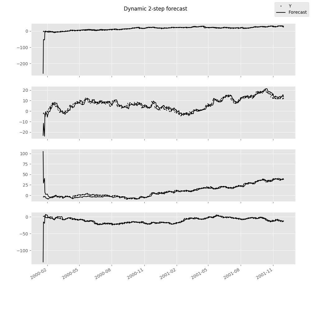
Dynamic forecasts for a given number of steps ahead can be produced using the
forecast function and return a pandas.DataMatrix object:
In [41]: var.forecast(2)
Out[41]:
                     A          B           C           D
2000-01-20 -260.325888 -23.141610  104.930427 -134.489882
2000-01-21  -52.121483 -11.566786   29.383608  -15.099109
2000-01-24  -54.900049 -23.894858   40.470913  -19.199059
2000-01-25   -7.493484  -4.057529    6.682707    4.301623
2000-01-26   -6.866108  -5.065873    5.623590    0.796081
...                ...        ...         ...         ...
2001-11-26   31.886126  13.515527   37.618145  -11.464682
2001-11-27   32.314633  14.237672   37.397691  -12.809727
2001-11-28   30.896528  15.488388   38.541596  -13.129524
2001-11-29   30.077228  15.533337   38.734096  -12.900891
2001-11-30   30.510380  13.491615   38.088228  -12.384976

[487 rows x 4 columns]
The forecasts can be visualized using plot_forecast:
In [42]: var.plot_forecast(2)
Class Reference
var_model.VAR(endog[, exog, dates, freq, …]) |
Fit VAR(p) process and do lag order selection |
var_model.VARProcess(coefs, coefs_exog, sigma_u) |
Class represents a known VAR(p) process |
var_model.VARResults(endog, endog_lagged, …) |
Estimate VAR(p) process with fixed number of lags |
irf.IRAnalysis(model[, P, periods, order, …]) |
Impulse response analysis class. |
var_model.FEVD(model[, P, periods]) |
Compute and plot Forecast error variance decomposition and asymptotic standard errors |
dynamic.DynamicVAR(data[, lag_order, …]) |
Estimates time-varying vector autoregression (VAR(p)) using equation-by-equation least squares |